How formulas work
Now we’ll describe the full nitty-gritty of how formulas are parsed and interpreted. Here’s the picture you’ll want to keep in mind:
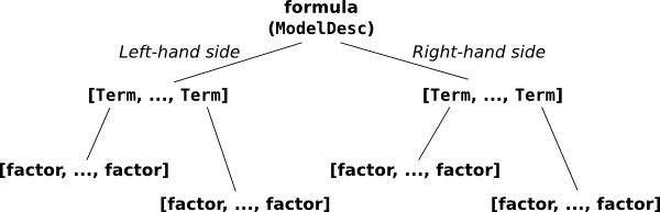
The pieces that make up a formula.
Say we have a formula like:
y ~ a + a:b + np.log(x)
This overall thing is a formula, and it’s divided into a left-hand
side, y, and a right-hand side, a + a:b +
np.log(x). (Sometimes you want a formula that has no left-hand
side, and you can write that as ~ x1 + x2 or even x1 + x2.)
Each side contains a list of terms separated by +; on the left
there is one term, y, and on the right, there are four terms:
a and a:b and np.log(x), plus an invisible intercept
term. And finally, each term is the interaction of zero or more
factors. A factor is the minimal, indivisible unit that each
formula is built up out of; the factors here are y, a, b,
and np.log(x). Most of these terms have only one factor – for
example, the term y is a kind of trivial interaction between the
factor y and, well… and nothing. There’s only one factor in that
“interaction”. The term a:b is an interaction between two factors,
a and b. And the intercept term is an interaction between
zero factors. (This may seem odd, but it turns out that defining the
zero-order interaction to produce a column of all ones is very
convenient, just like it turns out to be convenient to define the
product of an empty list to be np.prod([]) ==
1.)
Note
In the context of Patsy, the word factor does not refer specifically to categorical data. What we call a “factor” can represent either categorical or numerical data. Think of factors like in multiplying factors together, not like in factorial design. When we want to refer to categorical data, this manual and the Patsy API use the word “categorical”.
To make this more concrete, here’s how you could manually construct the same objects that Patsy will construct if given the above formula:
from patsy import ModelDesc, Term, EvalFactor
ModelDesc([Term([EvalFactor("y")])],
          [Term([]),
           Term([EvalFactor("a")]),
           Term([EvalFactor("a"), EvalFactor("b")]),
           Term([EvalFactor("np.log(x)")])
           ])
Compare to what you get from parsing the above formula:
ModelDesc.from_formula("y ~ a + a:b + np.log(x)")
ModelDesc represents an overall formula; it just takes two
lists of Term objects, representing the left-hand side and
the right-hand side. And each Term object just takes a list of
factor objects. In this case our factors are of type
EvalFactor, which evaluates arbitrary Python code, but in
general any object that implements the factor protocol will do – for
details see Model specification for experts and computers.
Of course as a user you never have to actually touch
ModelDesc, Term, or EvalFactor objects by
hand – but it’s useful to know that this lower layer exists in case
you ever want to generate a formula programmatically, and to have an
image in your mind of what a formula really is.
The formula language
Now let’s talk about exactly how those magic formula strings are processed.
Since a term is nothing but a set of factors, and a model is nothing
but two sets of terms, you can write any Patsy model just using
: to create interactions, + to join terms together into a set,
and ~ to separate the left-hand side from the right-hand side.
But for convenience, Patsy also understands a number of other
short-hand operators, and evaluates them all using a full-fledged
parser
complete with robust error reporting, etc.
Operators
The built-in binary operators, ordered by precedence, are:
~ |
lowest precedence (binds most loosely) |
+, - |
|
*, / |
|
: |
|
** |
highest precedence (binds most tightly) |
Of course, you can override the order of operations using
parentheses. All operations are left-associative (so a - b - c means
the same as (a - b) - c, not a - (b - c)). Their meanings are as
follows:
~- Separates the left-hand side and right-hand side of a formula. Optional. If not present, then the formula is considered to contain a right-hand side only.
+- Takes the set of terms given on the left and the set of terms given
on the right, and returns a set of terms that combines both (i.e.,
it computes a set union). Note that this means that
a +
a
is justa. -- Takes the set of terms given on the left and removes any terms which are given on the right (i.e., it computes a set difference).
*a * bis short-hand fora + b + a:b, and is useful for the common case of wanting to include all interactions between a set of variables while partitioning their variance between lower- and higher-order interactions. Standard ANOVA models are of the forma * b * c * ..../- This one is a bit quirky.
a / bis shorthand fora + a:b, and is intended to be useful in cases where you want to fit a standard sort of ANOVA model, butbis nested withina, soa*bdoesn’t make sense. So far so good. Also, if you have multiple terms on the right, then the obvious thing happens:a / (b + c)is equivalent toa + a:b + a:c(/is rightward distributive over+). But, if you have multiple terms on the left, then there is a surprising special case:(a + b)/cis equivalent toa + b + a:b:c(and note that this is different from what you’d get out ofa/c + b/c–/is not leftward distributive over+). Again, this is motivated by the idea of using this for nested variables. It doesn’t make sense forcto be nested within bothaandbseparately, unlessbis itself nested ina– but if that were true, then you’d writea/b/cinstead. So if we see(a + b)/c, we decide thataandbmust be independent factors, but thatcis nested within each combination of levels ofaandb, which is whata:b:cgives us. If this is confusing, then my apologies… S has been working this way for >20 years, so it’s a bit late to change it now. :- This takes two sets of terms, and computes the interaction between
each term on the left and each term on the right. So, for example,
(a + b):(c + d)is the same asa:c + a:d + b:c + b:d. Calculating the interaction between two terms is also a kind of set union operation, but:takes the union of factors within two terms, while+takes the union of two sets of terms. Note that this means thata:ais justa, and(a:b):(a:c)is the same asa:b:c. **This takes a set of terms on the left, and an integer n on the right, and computes the
*of that set of terms with itself n times. This is useful if you want to compute all interactions up to order n, but no further. Example:(a + b + c + d) ** 3
is expanded to:
(a + b + c + d) * (a + b + c + d) * (a + b + c + d)
Note that an equivalent way to write this particular expression would be:
a*b*c*d - a:b:c:d
(Exercise: why?)
The parser also understands unary + and -, though they aren’t very
useful. + is a no-op, and - can only be used in the forms -1
(which means the same as 0) and -0 (which means the same as
1). See below for more on 0 and
1.
Factors and terms
So that explains how the operators work – the verbs in the formula
language – but what about the nouns, the terms like y and
np.log(x) that are actually picking out bits of your data?
Individual factors are allowed to be arbitrary Python code. Scanning
arbitrary Python code can be quite complicated, but Patsy uses the
official Python tokenizer that’s built into the standard library, so
it’s able to do it robustly. There is still a bit of a problem,
though, since Patsy operators like + are also valid Python
operators. When we see a +, how do we know which interpretation to
use?
The answer is that a Python factor begins whenever we see a token which
- is not a Patsy operator listed in that table up above, and
- is not a parenthesis
And then the factor ends whenever we see a token which
- is a Patsy operator listed in that table up above, and
- it not enclosed in any kind of parentheses (where “any kind” includes regular, square, and curly bracket varieties)
This will be clearer with an example:
f(x1 + x2) + x3
First, we see f, which is not an operator or a parenthesis, so we
know this string begins with a Python-defined factor. Then we keep
reading from there. The next Patsy operator we see is the + in
x1 + x2… but since at this point we have seen the opening (
but not the closing ), we know that we’re inside parentheses and
ignore it. Eventually we come to the second +, and by this time we
have seen the closing parentheses, so we know that this is the end of
the first factor and we interpret the + as a Patsy operator.
One side-effect of this is that if you do want to perform some
arithmetic inside your formula object, you can hide it from the
Patsy parser by putting it inside a function call. To make this
more convenient, Patsy provides a builtin function I()
that simply returns its input. (Hence the name: it’s the Identity
function.) This means you can use I(x1 + x2) inside a formula to
represent the sum of x1 and x2.
Note
The above plays a bit fast-and-loose with the distinction
between factors and terms. If you want to get more technical, then
given something like a:b, what’s happening is first that we
create a factor a and then we package it up into a
single-factor term. And then we create a factor b, and we
package it up into a single-factor term. And then we evaluate the
:, and compute the interaction between these two terms. When
we encounter embedded Python code, it’s always converted straight
to a single-factor term before doing anything else.
Intercept handling
There are two special things about how intercept terms are handled inside the formula parser.
First, since an intercept term is an interaction of zero factors, we
have no way to write it down using the parts of the language described
so far. Therefore, as a special case, the string 1 is taken to
represent the intercept term.
Second, since intercept terms are almost always wanted and remembering
to include them by hand all the time is quite tedious, they are always
included by default in the right-hand side of any formula. The way
this is implemented is exactly as if there is an invisible 1 +
inserted at the beginning of every right-hand side.
Of course, if you don’t want an intercept, you can remove it again
just like any other unwanted term, using the - operator. The only
thing that’s special about the 1 + is that it’s invisible;
otherwise it acts just like any other term. This formula has an
intercept:
y ~ x
because it is processed like y ~ 1 + x.
This formula does not have an intercept:
y ~ x - 1
because it is processed like y ~ 1 + x - 1.
Of course if you want to be really explicit you can mention the intercept explicitly:
y ~ 1 + x
Once the invisible 1 + is added, this formula is processed like
y ~ 1 + 1 + x, and as you’ll recall from the definition of +
above, adding the same term twice produces the same result as adding
it just once.
For compatibility with S and R, we also allow the magic terms 0 and
-1 which represent the “anti-intercept”. Adding one of these terms
has exactly the same effect as subtracting the intercept term, and
subtracting one of these terms has exactly the same effect as adding
the intercept term. That means that all of these formulas are
equivalent:
y ~ x - 1
y ~ x + -1
y ~ -1 + x
y ~ 0 + x
y ~ x - (-0)
Explore!
The formula language is actually fairly simple once you get the hang of it, but if you’re ever in doubt as to what some construction means, you can always ask Patsy how it expands.
Here’s some code to try out at the Python prompt to get started:
from patsy import ModelDesc
ModelDesc.from_formula("y ~ x")
ModelDesc.from_formula("y ~ x + x + x")
ModelDesc.from_formula("y ~ -1 + x")
ModelDesc.from_formula("~ -1")
ModelDesc.from_formula("y ~ a:b")
ModelDesc.from_formula("y ~ a*b")
ModelDesc.from_formula("y ~ (a + b + c + d) ** 2")
ModelDesc.from_formula("y ~ (a + b)/(c + d)")
ModelDesc.from_formula("np.log(x1 + x2) "
                       "+ (x + {6: x3, 8 + 1: x4}[3 * i])")
Sometimes it might be easier to read if you put the processed formula
back into formula notation using ModelDesc.describe():
desc = ModelDesc.from_formula("y ~ (a + b + c + d) ** 2")
desc.describe()
From terms to matrices
So at this point, you hopefully understand how a string is parsed into
the ModelDesc structure shown in the figure at the top of
this page. And if you like you can also produce such structures
directly without going through the formula parser (see
Model specification for experts and computers). But these terms and factors
objects are still a fairly high-level, symbolic representation of a
model. Now we’ll talk about how they get converted into actual
matrices with numbers in.
There are two core operations here. The first takes a list of
Term objects (a termlist) and some data, and produces a
DesignMatrixBuilder. The second takes a
DesignMatrixBuilder and some data, and produces a design
matrix. In practice, these operations are implemented by
design_matrix_builders() and build_design_matrices(),
respectively, and each of these functions is “vectorized” to process
an arbitrary number of matrices together in a single operation. But
we’ll ignore that for now, and just focus on what happens to a single
termlist.
First, each individual factor is given a chance to set up any Stateful transforms it may have, and then is evaluated on the data, to determine:
- Whether it is categorical or numerical
- If it is categorical, what levels it has
- If it is numerical, how many columns it has.
Next, we sort terms based on the factors they contain. This is done by dividing terms into groups based on what combination of numerical factors each one contains. The group of terms that have no numerical factors comes first, then the rest of the groups in the order they are first mentioned within the term list. Then within each group, lower-order interactions are ordered to come before higher-order interactions. (Interactions of the same order are left alone.)
Example:
In [1]: data = demo_data("a", "b", "x1", "x2")

In [2]: mat = dmatrix("x1:x2 + a:b + b + x1:a:b + a + x2:a:x1", data)

In [3]: mat.design_info.term_names
Out[3]: ['Intercept', 'b', 'a', 'a:b', 'x1:x2', 'x2:a:x1', 'x1:a:b']
The non-numerical terms are Intercept, b, a, a:b and they come first, sorted from lower-order to higher-order. b comes before a because it did in the original formula. Next come the terms that involved x1 and x2 together, and x1:x2 comes before x2:a:x1 because it is a lower-order term. Finally comes the sole term involving x1 without x2.
Note
These ordering rules may seem a bit arbitrary, but will make more sense after our discussion of redundancy below. Basically the motivation is that terms like b and a represent overlapping vector spaces, which means that the presence of one will affect how the other is coded. So, we group to them together, to make these relationships easier to see in the final analysis. And, a term like b represents a sub-space of a term like a:b, so if you’re including both terms in your model you presumably want the variance represented by b to be partitioned out separately from the overall a:b term, and for that to happen, b should come first in the final model.
After sorting the terms, we determine appropriate coding schemes for
categorical factors, as described in the next section. And that’s it
– we now know exactly how to produce this design matrix, and
design_matrix_builders() packages this knowledge up into a
DesignMatrixBuilder and returns it. To get the design matrix
itself, we then use build_design_matrices().
Redundancy and categorical factors
Here’s the basic idea about how Patsy codes categorical factors: each
term that’s included means that we want our outcome variable to be
able to vary in a certain way – for example, the a:b in y ~ a:b
means that we want our model to be flexible enough to assign y a
different value for every possible combination of a and b
values. So what Patsy does is build up a design matrix incrementally
by working from left to right in the sorted term list, and for each
term it adds just the right columns needed to make sure that the model
will be flexible enough to include the kind of variation this term
represents, while keeping the overall design matrix full rank. The
result is that the columns associated with each term always represent
the additional flexibility that the models gains by adding that
term, on top of the terms to its left. Numerical factors are assumed
not to be redundant with each other, and are always included “as is”;
categorical factors and interactions might be redundant, so Patsy
chooses either full-rank or reduced-rank contrast coding for each one
to keep the overall design matrix at full rank.
Note
We’re only worried here about “structural redundancies”, those which occur inevitably no matter what the particular values occur in your data set. If you enter two different factors x1 and x2, but set them to be numerically equal, then Patsy will indeed produce a design matrix that isn’t full rank. Avoiding that is your problem.
Okay, now for the more detailed explanation. Each term represents a certain space of linear combinations of column vectors:
- A numerical factor represents the vector space spanned by its columns.
- A categorical factor represents the vector space spanned by the columns you get if you apply “dummy coding”.
- An interaction between two factors represents the vector space
spanned by the element-wise products between vectors in the first
factor’s space with vectors in the second factor’s space. For
example, if
 and
and  are two columns that
form a basis for the vector space represented by factor
are two columns that
form a basis for the vector space represented by factor  ,
and likewise
,
and likewise  and
and  are a basis for the
vector space represented by
are a basis for the
vector space represented by  , then
  ,
,  ,
,  ,
,
 is a basis for the vector space represented
by
is a basis for the vector space represented
by  . Here the
  operator represents
elementwise multiplication, like numpy
operator represents
elementwise multiplication, like numpy *. (Exercise: show that the choice of basis does not matter.) - The empty interaction represents the space spanned by the identity element for elementwise multiplication, i.e., the all-ones “intercept” term.
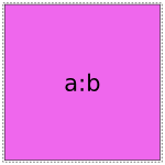
So suppose that a is a categorical factor with two levels a1 and a2, and b is a categorical factor with two levels b1 and b1. Then:
a represents the space spanned by two vectors: one that has a 1 everywhere that
a == "a1", and a zero everywhere else, and another that’s similar but fora == "a2". (dummy coding)b works similarly
and a:b represents the space spanned by four vectors: one that has a 1 everywhere that has
a == "a1"andb == "b1", another that has a 1 everywhere that hasa1 == "a2"andb == "b1", etc. So if you are familiar with ANOVA terminology, then these are not the kinds of interactions you are expecting! They represent a more fundamental idea, that when we write:y ~ a:b
we mean that the value of y can vary depending on every possible combination of a and b.

Notice that this means that the space spanned by the intercept term is always a vector subspace of the spaces spanned by a and b, and these subspaces in turn are always subspaces of the space spanned by a:b. (Another way to say this is that a and b are “marginal to” a:b.) The diagram on the right shows these relationships graphically. This reflects the intuition that allowing y to depend on every combination of a and b gives you a more flexible model than allowing it to vary based on just a or just b.
So what this means is that once you have a:b in your model, adding a or b or the intercept term won’t actually give you any additional flexibility; the most they can do is to create redundancies that your linear algebra package will have to somehow detect and remove later. These two models are identical in terms of how flexible they are:
y ~ 0 + a:b
y ~ 1 + a + b + a:b
And, indeed, we can check that the matrices that Patsy generates for these two formulas have identical column spans:
In [4]: data = demo_data("a", "b", "y")

In [5]: mat1 = dmatrices("y ~ 0 + a:b", data)[1]

In [6]: mat2 = dmatrices("y ~ 1 + a + b + a:b", data)[1]

In [7]: np.linalg.matrix_rank(mat1)
Out[7]: 4

In [8]: np.linalg.matrix_rank(mat2)
Out[8]: 4

In [9]: np.linalg.matrix_rank(np.column_stack((mat1, mat2)))
Out[9]: 4
But, of course, their actual contents are different:
In [10]: mat1
Out[10]:
DesignMatrix with shape (8, 4)
  a[a1]:b[b1]  a[a2]:b[b1]  a[a1]:b[b2]  a[a2]:b[b2]
            1            0            0            0
            0            0            1            0
            0            1            0            0
            0            0            0            1
            1            0            0            0
            0            0            1            0
            0            1            0            0
            0            0            0            1
  Terms:
    'a:b' (columns 0:4)

In [11]: mat2
Out[11]:
DesignMatrix with shape (8, 4)
  Intercept  a[T.a2]  b[T.b2]  a[T.a2]:b[T.b2]
          1        0        0                0
          1        0        1                0
          1        1        0                0
          1        1        1                1
          1        0        0                0
          1        0        1                0
          1        1        0                0
          1        1        1                1
  Terms:
    'Intercept' (column 0)
    'a' (column 1)
    'b' (column 2)
    'a:b' (column 3)
This happens because Patsy is finding ways to avoid creating
redundancy while coding each term. To understand how this works, it’s
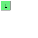
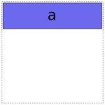
useful to draw some pictures. Patsy has two general strategies for
coding a categorical factor with  levels. The first is to use
a full-rank encoding with columns. Here are some pictures of
this style of coding:
levels. The first is to use
a full-rank encoding with columns. Here are some pictures of
this style of coding:
Obviously if we lay these images on top of each other, they’ll overlap, which corresponds to their overlap when considered as vector spaces. If we try just putting them all into the same model, we get mud:
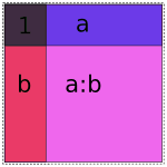
Naive 1 + a + b + a:b
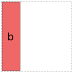
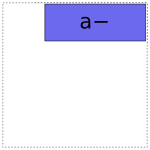
Patsy avoids this by using its second strategy: coding an
level factor in  columns which, critically, do not span
the intercept. We’ll call this style of coding reduced-rank, and use
notation like a- to refer to factors coded this way.
columns which, critically, do not span
the intercept. We’ll call this style of coding reduced-rank, and use
notation like a- to refer to factors coded this way.
Note
Each of the categorical coding schemes included in patsy
come in both full-rank and reduced-rank flavours. If you ask for,
say, Poly coding, then this is the mechanism used to
decide whether you get full- or reduced-rank Poly coding.
For coding a there are two options:
And likewise for b:
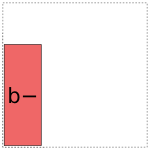
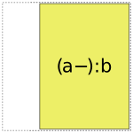
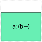
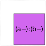
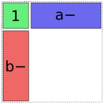
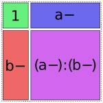
When it comes to a:b, things get more interesting: it can choose whether to use a full- or reduced-rank encoding separately for each factor, leading to four choices overall:
So when interpreting a formula like 1 + a + b + a:b, Patsy’s
job is to pick and choose from the above pieces and then assemble them
together like a jigsaw puzzle.
Let’s walk through the formula 1 + a + b + a:b to see how this
works. First it encodes the intercept:
In [12]: dmatrices("y ~ 1", data)[1]
Out[12]:
DesignMatrix with shape (8, 1)
  Intercept
          1
          1
          1
          1
          1
          1
          1
          1
  Terms:
    'Intercept' (column 0)
Then it adds the a term. It has two choices, either the full-rank coding or the reduced rank a- coding. Using the full-rank coding would overlap with the already-existing intercept term, though, so it chooses the reduced rank coding:
In [13]: dmatrices("y ~ 1 + a", data)[1]
Out[13]:
DesignMatrix with shape (8, 2)
  Intercept  a[T.a2]
          1        0
          1        0
          1        1
          1        1
          1        0
          1        0
          1        1
          1        1
  Terms:
    'Intercept' (column 0)
    'a' (column 1)
The b term is treated similarly:
In [14]: dmatrices("y ~ 1 + a + b", data)[1]
Out[14]:
DesignMatrix with shape (8, 3)
  Intercept  a[T.a2]  b[T.b2]
          1        0        0
          1        0        1
          1        1        0
          1        1        1
          1        0        0
          1        0        1
          1        1        0
          1        1        1
  Terms:
    'Intercept' (column 0)
    'a' (column 1)
    'b' (column 2)
And finally, there are four options for the a:b term, but only one of them will fit without creating overlap:
In [15]: dmatrices("y ~ 1 + a + b + a:b", data)[1]
Out[15]:
DesignMatrix with shape (8, 4)
  Intercept  a[T.a2]  b[T.b2]  a[T.a2]:b[T.b2]
          1        0        0                0
          1        0        1                0
          1        1        0                0
          1        1        1                1
          1        0        0                0
          1        0        1                0
          1        1        0                0
          1        1        1                1
  Terms:
    'Intercept' (column 0)
    'a' (column 1)
    'b' (column 2)
    'a:b' (column 3)
Patsy tries to use the fewest pieces possible to cover the space. For instance, in this formula, the a:b term is able to fill the remaining space by using a single piece:
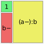
In [16]: dmatrices("y ~ 1 + b + a:b", data)[1]
Out[16]:
DesignMatrix with shape (8, 4)
  Intercept  b[T.b2]  a[T.a2]:b[b1]  a[T.a2]:b[b2]
          1        0              0              0
          1        1              0              0
          1        0              1              0
          1        1              0              1
          1        0              0              0
          1        1              0              0
          1        0              1              0
          1        1              0              1
  Terms:
    'Intercept' (column 0)
    'b' (column 1)
    'a:b' (columns 2:4)
However, this is not always possible. In such cases, Patsy will assemble multiple pieces to code a single term [1], e.g.:
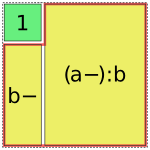
In [17]: dmatrices("y ~ 1 + a:b", data)[1]
Out[17]:
DesignMatrix with shape (8, 4)
  Intercept  b[T.b2]  a[T.a2]:b[b1]  a[T.a2]:b[b2]
          1        0              0              0
          1        1              0              0
          1        0              1              0
          1        1              0              1
          1        0              0              0
          1        1              0              0
          1        0              1              0
          1        1              0              1
  Terms:
    'Intercept' (column 0)
    'a:b' (columns 1:4)
Notice that the matrix entries and column names here are identical to those produced by the previous example, but the association between terms and columns shown at the bottom is different.
In all of these cases, the final model spans the same space; a:b is included in the formula, and therefore the final matrix must fill in the full a:b square. By including different combinations of lower-order interactions, we can control how this overall variance is partitioned into distinct terms.
Exercise: create the similar diagram for a formula that includes a three-way interaction, like1 + a + a:b + a:b:cor1 + a:b:c. Hint: it’s a cube. Then, send us your diagram for inclusion in this documentation [2].
Finally, we’ve so far only discussed purely categorical interactions. Bringing numerical interactions into the mix doesn’t make things much more complicated. Each combination of numerical factors is considered to be distinct from all other combinations, so we divide all of our terms into groups based on which numerical factors they contain (just like we do when sorting terms, as described above), and then within each group we separately apply the algorithm described here to the categorical parts of each term.
Technical details
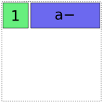
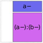
The actual algorithm Patsy uses to produce the above coding is very simple. Within the group of terms associated with each combination of numerical factors, it works from left to right. For each term it encounters, it breaks the categorical part of the interaction down into minimal pieces, e.g. a:b is replaced by 1 + (a-) + (b-) + (a-):(b-):
(Formally speaking, these “minimal pieces” consist of the set of all subsets of the original interaction.) Then, any of the minimal pieces which were used by a previous term within this group are deleted, since they are redundant:
and then we greedily recombine the pieces that are left by repeatedly merging adjacent pieces according to the rule ANYTHING + ANYTHING : FACTOR- = ANYTHING : FACTOR:
Exercise: Prove formally that the space spanned by ANYTHING + ANYTHING : FACTOR- is identical to the space spanned by ANYTHING : FACTOR.
Exercise: Either show that the greedy algorithm here produces optimal encodings in some sense (e.g., smallest number of pieces used), or else find a better algorithm. (Extra credit: implement your algorithm and submit a pull request [3].)
Is this algorithm correct? A full formal proof would be too tedious for this reference manual, but here’s a sketch of the analysis.
Recall that our goal is to maintain two invariants: the design matrix column space should include the space associated with each term, and should avoid “structural redundancy”, i.e. it should be full rank on at least some data sets. It’s easy to see the above algorithm will never “lose” columns, since the only time it eliminates a subspace is when it has previously processed that exact subspace within the same design. But will it always detect all the redundancies that are present?
That is guaranteed by the following theorem:
Theorem: Let two sets of factors,  and
and
 be given, and let
  be the numerical and categorical
factors, respectively (and similarly for
be the numerical and categorical
factors, respectively (and similarly for 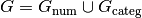 . Then the space represented by the interaction
 has a non-trivial intersection with the
space represented by the interaction
has a non-trivial intersection with the
space represented by the interaction  whenever:
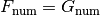 , and
, and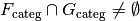
And, furthermore, whenever this condition does not hold, then there exists some assignment of values to the factors for which the associated vector spaces have only a trivial intersection.
Exercise: Prove it.
Exercise: Show that given a sufficient number of rows, the set of factor assignments on which
without the above conditions being satisfied is actually a zero set.
Corollary: Patsy’s strategy of dividing into groups by numerical factors, and then comparing all subsets of the remaining categorical factors, allows it to precisely identify and avoid structural redundancies.
Footnotes
| [1] | This is one of the places where Patsy improves on R, which produces incorrect output in this case (see Differences between R and Patsy formulas). |
| [2] | Yes, I’m lazy. And shameless. |
| [3] | Yes, still shameless. |